Introduction to Complete Knapsack Problem

ACMer

13 years ago

In [here], the basic 0/1 knapsack is discussed. For each item, you can choose to put or not to put into the knapsack. Therefore, for the number of items, there are only two options: 0 or 1.

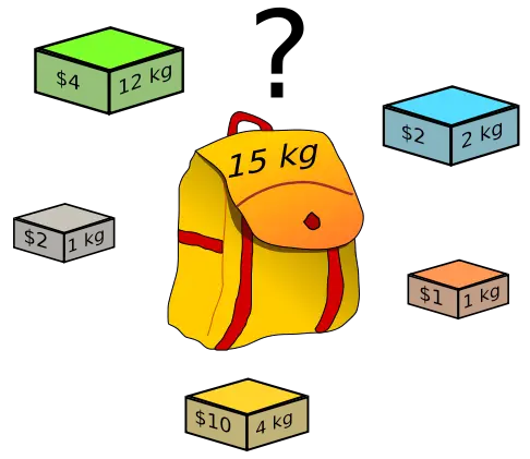
In Complete Knapsack Problem, for each item, you can put as many times as you want. Therefore, if capacity allows, you can put 0, 1, 2, items for each type. The Complete Knapsack Problem can also be modelling using 0/1 Knapsack.
>

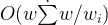
Similar to 0/1 Knapsack, there are O(WN) states that need to be computed. However, for the 0/1 knapsack, the complexity of solving each state is constant. The Complete Knapsack needs for each state. The total complexity can be considered as

One greedy optimisation is to replace items of heavier-but-less-valuable items with ones of lighter-more-valuable. If and we can simply and safely use item j instead of item i. This optimisation process can be done in time.

Another straightforward transform to 0/1 Knapsack Problem is to consider the maximum number of times for item i to put is . Therefore, we can treat item i as [/math] w / w_i [/math] items that are of same weight w_i. This does not increase time complexity: by simply splitting one item into many.

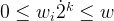
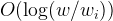
The other better transform is to split item i to items that have weights and values for . This is based on binary. No matter how many items we choose, we can represent the total number as the sum of many sub-items. This splitting yields .